2. Connecting your own model
The design optimization and uncertainty quantification algorithms are introduced on hydrogen-based energy systems. However, RHEIA algorithms can be applied on any system model, thus allowing to evaluate and connect your own model. In this section, first, the Python wrapper is described, which connects the system model with the optimization and uncertainty quantification algorithms. Thereafter, the connection of a Python-based model and a closed-source model is described.
2.1. Python wrapper
The Python wrapper module case_description enables to connect the system model to the uncertainty quantification and optimization algorithms.
The module includes two functions: set_params() and evaluate().
In set_params(), data can be imported before the model evaluations commence.
In this way, the computational cost of importing data is spent only once,
before the evaluation loop.
To illustrate, importing data from 3 data files (e.g. datafile_1.csv, datafile_2.csv, datafile_3.csv)
can be defined as follows in the case_description module:
import pandas as pd

def set_params():
    path = os.path.dirname(os.path.abspath(__file__))

    data1 = pd.read_csv(os.path.join(path, 'datafile_1.csv'))['data1']
    data2 = pd.read_csv(os.path.join(path, 'datafile_2.csv'))['data2']
    data3 = pd.read_csv(os.path.join(path, 'datafile_3.csv'))['data3']

    params = [data1, data2, data3]

    return params
The model evaluation is performed in the function evaluate(). This function is called
by the optimization algorithm or uncertainty quantification algorithm,
which provides the sample as an argument in the form of an enumerate object x.
The keys of the dictionary x[1] consist of the model parameter names and design variable names,
as defined in design_space.csv and stochastic_space.csv.
The corresponding values are the values generated by the optimization or uncertainty quantification algorithm.
In addition to the enumerate object x, the evaluate() function takes params as an optional argument.
This list contains the list with imported data, as returned by the function set_params().
When set_params() does not exist, i.e. when no data needs to be imported before the model evaluations commence,
params corresponds to an empty list.
In summary, the evaluate() function can be defined as follows:
def evaluate(x_in, params = []):

    arguments = params + [x_in[1]]

    obj_1, obj_2 = system_model_evaluation(*arguments)

    return obj_1, obj_2
2.2. Four-bar truss Python model
To illustrate the connection of a Python-based model to RHEIA, a model of a four-bar truss is adopted. First, the system is briefly illustrated, followed by the model connection and the optimization commands.
2.2.1. Four-bar truss system description
The four-bar truss is presented below:
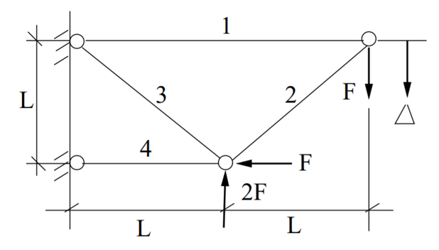
The four-bar truss
The aim is to minimize the volume of the truss and to minimize the deflection of the outermost joint by controlling the cross-sectional areas of the bars. The volume \(V\) and deflection \(d\) are defined as:
\(V = L (2A_1 + \sqrt{2} A_2 + \sqrt{A_3} + A_4 )\)
\(d = F L \left( \dfrac{2}{A_1 E_1} + \dfrac{2 \sqrt{2}}{A_2 E_2} - \dfrac{2 \sqrt{2}}{A_3 E_3} + \dfrac{2}{A_4} \right)\)
Where \(F,~L,~E,~A\) are the exerted force, length, Young’s modulus and cross-sectional area, respectively. The cross-sectional areas are designed respecting the following bounds:
\(A_1 \in [1,3] ~\mathrm{cm}^2\)
\(A_2 \in [\sqrt{2},3] ~\mathrm{cm}^2\)
\(A_3 \in [\sqrt{2},3] ~\mathrm{cm}^2\)
\(A_4 \in [1,3] ~\mathrm{cm}^2\)
And the model parameters are defined as follows:
\(L = 200 ~ \mathrm{cm}^2\)
\(F \in \mathcal{N}(10,1) ~ \mathrm{kN}\)
\(E_1 \in \mathcal{U}(19000,21000) ~ \mathrm{kN}/ \mathrm{cm}^2\)
\(E_2 \in \mathcal{U}(19000,21000) ~ \mathrm{kN}/ \mathrm{cm}^2\)
\(E_3 \in \mathcal{U}(19000,21000) ~ \mathrm{kN}/ \mathrm{cm}^2\)
\(E_4 \in \mathcal{U}(19000,21000) ~ \mathrm{kN}/ \mathrm{cm}^2\)
Conclusively, the system model evaluation is coded as follows:
def four_bar_truss(x_i):

    vol = x_i['L'] * (2. * x_i['A_1'] + 2.**(0.5) *
                      x_i['A_2'] + x_i['A_3']**(0.5) + x_i['A_4'])

    disp = x_i['F'] * x_i['L'] * (2. / (x_i['A_1'] * x_i['E_1']) +
                                  2. * 2**(0.5) / (x_i['A_2'] * x_i['E_2']) -
                                  2. * 2**(0.5) / (x_i['A_3'] * x_i['E_3']) +
                                  2. / (x_i['A_4'] * x_i['E_4']))

    return vol, disp
Where the function argument x is a dictionary with values for the model parameters, i.e. \(L,~F,~E_1,~E_2,~E_3,~E_4\),
and values for the design variables, i.e. \(A_1,~A_2,~A_3,~A_4\).
This function is located in the four_bar_truss module.
2.2.2. Connecting the case to the framework
To connect the model to the optimization and uncertainty quantification framework, a specific folder for the model
should be created in the general CASES folder. In the CASES folder, a reference folder CASES\REF is present, which includes the necessary
files to characterize and connect a new system model.
Make a copy of the REF folder, paste it in the CASES folder and rename it, e.g. into FOUR_BAR_TRUSS.
Hence, a new case folder is present: CASES\FOUR_BAR_TRUSS.
This folder includes design_space.csv, stochastic_space.csv and case_description.
Finally, include the four_bar_truss module in the folder.
The FOUR_BAR_TRUSS folder now includes all necessary files and the structure looks as follows:
CASES
    FOUR_BAR_TRUSS
        design_space.csv
        stochastic_space.csv
        case_despcription.py
        four_bar_truss.py
In design_space.csv, the design variables and model parameters are defined.
More information on the characterization of the design space is presented in The design_space.csv file.
In the four-bar truss example, 4 design variables (the cross-sectional areas) and 6 model parameters (the force, length and 4 Young’s moduli) exist.
The corresponding design_space.csv file for the four-bar truss is configured as:
A_1 var 1 3
A_2 var 1.414 3
A_3 var 1.414 3
A_4 var 1 3
L   par 200
F   par 10
E_1 par 20000
E_2 par 20000
E_3 par 20000
E_4 par 20000
The uncertainty on the stochastic parameters should be defined in stochastic_space.csv.
More information on the uncertainty characterization is described in The stochastic_space.csv file.
The exerted force and the Young’s moduli are subject to uncertainty.
The corresponding stochastic_space.csv file for the four-bar truss file is configured as:
F   absolute Gaussian 1
E_1 absolute Uniform  1000
E_2 absolute Uniform  1000
E_3 absolute Uniform  1000
E_4 absolute Uniform  1000
To evaluate the system model in the optimization and uncertainty quantification algorithm, the model should be
connected to the algorithms. This connection is established in the module case_description.
Additional details on this module are provided in Python wrapper.
At the top of the file, import the module or function that evaluates your model. In the example of the four-bar truss,
this is performed as follows:
from rheia.CASES.FOUR_BAR_TRUSS.four_bar_truss import four_bar_truss
After the import, the model can be evaluated. This is done in the evaluate() function.
The dictionary with the input sample names and values x[1] is passed directly as an argument to the four_bar_truss() function.
The four_bar_truss() function returns the values for the optimization objectives, i.e. the volume \(V\) and deflection \(d\).
Conclusively, the evaluate() function is completed as follows:
def evaluate(x_in, params = []):

    vol, disp = four_bar_truss(x_in[1])

    return vol, disp
2.2.3. Run a design optimization
Once the characterization and coupling of the case is completed, the optimization dictionary can be completed to perform the design optimization. To illustrate, for a deterministic design optimization:
 1import rheia.OPT.optimization as rheia_opt
 2
 3dict_opt = {'case':                'FOUR_BAR_TRUSS',
 4            'objectives':          {'DET': (-1, -1)},
 5            'stop':                ('BUDGET', 9000),
 6            'population size':     30,
 7            'results dir':         'run_1',
 8           }
 9
10rheia_opt.run_opt(dict_opt)
In this dictionary, a deterministic design optimization is specified, for which both objectives should be minimized. The computational budget is set at 9000, which leads to at least 300 generations with a population size of 30. The number of jobs, crossover probability, mutation probability, eta, starting population and result printing are adopted from the standard setting and are therefore not specified in the dictionary. Similarly, the optimization dictionary for robust design optimization on the mean and standard deviation of the displacement can be characterized as follows:
 1import rheia.OPT.optimization as rheia_opt
 2
 3dict_opt = {'case':                  'FOUR_BAR_TRUSS',
 4            'objectives':            {'ROB': (-1, -1)},
 5            'stop':                  ('BUDGET', 90000),
 6            'population size':       30,
 7            'pol order':             2,
 8            'objective names':       ['V', 'd'],
 9            'objective of interest': ['d'],
10            'results dir':           'run_1',
11            }
12
13rheia_opt.run_opt(dict_opt)
The details on running optimization or uncertainty quantification are provided in Run an optimization task and Run an uncertainty quantification, respectively.
2.3. EnergyPLAN closed-source model
EnergyPLAN is a software that evaluates national energy system operation. It is used by industry, researchers and policy-makers worldwide. The software includes the electricity, heating, cooling, industry and transport sector to characterize, among others, the primary energy consumption and CO2 emissions. Generally, the software is used through a user-friendly user interface, but it can be called through an external command as well. When calling EnergyPLAN through an external command, the input parameters are provided and the outputs are written in external text files.
In this tutorial, the EnergyPLAN software is connected to the framework. The specific case is based on exercise 3 in the EnergyPLAN training session.
The energy system is characterized as follows:
Electricity demand: \(\mathrm{elec\_demand} \in \mathcal{U}(33.3,35.3) ~ \mathrm{TWh/year}\);
Condensing coal-fired power plant: 9000 MW;
On-shore wind power: 4000 MW;
Off-shore wind power: 3000 MW;
Annual district heating demand: 27.43 TWh (1.59 TWh district heating oil-boilers, 10 TWh small-scale CHP, 15.84 TWh large-scale CHP extraction plants);
Decentralised natural-gas fired CHP: 1350 MW, with a thermal efficiency of \(\mathrm{CHP\_eff\_ht} \in \mathcal{U}(0.45,0.55)\) and electrical efficiency of \(\mathrm{CHP\_eff\_el} \in \mathcal{U}(0.36,0.46)\);
Large-scale coal-fired CHP: 2000 MW, with a thermal efficiency of 50% and electrical efficiency of 41%;
Heat Pump of 300 MWe with a \(\mathrm{COP} \in \mathcal{U}(2.5,3.5)\);
Individual house Fuel demand for heating:14.42 TWh (0.01 coal, 4.2 oil, 5.66 natural gas and 4.55 biomass);
Industrial fuel demand: 53.66 TWh (3.37 coal, 26.92 oil, 18.19 natural gas and 5.18 biomass);
Industrial district heating production: 1.73 TWh;
Industrial district electricity production: 2.41 TWh;
Transportation fuel demand: 13.25 TWh Jet Petrol, 27.50 TWh Diesel, 23.35 TWh Petrol and 2.55 TWh hydrogen;
900 MWe electrolyzers at \(\mathrm{eff\_H2} \in \mathcal{U}(0.6,0.7)\) efficiency for hydrogen production for transport.
2.3.1. Connecting the model to the framework
First, a specific folder for the model should be created in the CASES folder, e.g. ENERGYPLAN.
The necessary files are design_space.csv, the case_description module( and stochastic_space.csv for uncertainty quantification and robust design optimization).
In addition, a module to call the EnergyPLAN software run_energyplan
and a .csv file to provide the input that represent the current case (case.csv) are included.
This results in the following structure:
CASES
    ENERGYPLAN
        design_space.csv
        stochastic_space.csv
        case_despcription.py
        run_energyplan.py
        case.csv
The design_space.csv file includes the mean values for the stochastic model parameters:
elec_demand par 34.3
COP         par 3
eff_H2      par 0.65
CHP_eff_el  par 0.41
CHP_eff_th  par 0.5
More information on the characterization of the design space is presented in The design_space.csv file.
The stochastic space is defined in stochastic_space.csv:
elec_demand absolute Uniform 1
COP         absolute Uniform 0.5
eff_H2      absolute Uniform 0.05
CHP_eff_el  absolute Uniform 0.05
CHP_eff_th  absolute Uniform 0.05
More information on the uncertainty characterization is described in The stochastic_space.csv file.
In the run_energyplan module, the energyplan() Python wrapper evaluates the EnergyPLAN model and returns the model outputs of interest.
In this function, first, the index and sample are splitted from the x_tup argument.
Then, the path of the energyPLAN.exe executable and the case.csv file with input parameters are provided:
x = x_tup[1]
index = x_tup[0]
path = os.path.dirname(os.path.abspath(__file__))

ep_path = r'C:\energyPLAN\energyPLAN.exe'
input_file = os.path.join(path, 'case.csv')
A new input file is created for the energyPLAN model,
where the initial values of the model parameters are overwritten by the new values, provided by the input sample x:
new_input_file = '%s_%i.csv' % (input_file[:-4], index)

create_new_input_file(input_file, new_input_file, x)
This new input file, with updated values on the model parameters for each evaluation, has a name that ends with the index of the input sample, i.e. the sample position in the array of samples created for uncertainty quantification. In this way, a unique input file is generated for each input sample, which ensures that during the parallelization of the model evaluations over the available CPUs, the input file that corresponds to the input sample is evaluated. Following a similar logic, the name of the file with results is defined as:
result_file = os.path.join(path, 'result_%i.csv' % index)
Once the EnergyPLAN input file is characterized, the command to run EnergyPLAN is called:
cm = [ep_path, '-i', new_input_file, '-ascii', result_file]
sp.call(cm)
Followed by reading the values for the quantities of interest:
co2, fuel = read_output_file(result_file)
We refer to the run_energyplan module for additional details on the create_new_input_file() and read_output_file() functions.
In the case_description module, the function to run the case in EnergyPLAN is imported from the run_energyplan() module at the top of the script:
from rheia.CASES.ENERGYPLAN.run_energyplan import energyplan
The run_energyplan() function is evaluated in evaluate(), where the enumerate object x_in is provided as an argument. For this case, no fixed parameters are provided as an argument:
def evaluate(x_in, params=[]):

    co2, fuel = energyplan(x_in)

    return co2, fuel
The enumerate object x_in contains the sample to be evaluated and the index of the sample in the list of samples.
2.3.2. Run uncertainty quantification
With the characterization complete for uncertainty quantification, the algorithm can be initiated with:
 1import rheia.UQ.uncertainty_quantification as rheia_uq
 2import multiprocessing as mp
 3
 4
 5dict_uq = {'case':                  'ENERGYPLAN',
 6           'n jobs':                int(mp.cpu_count() / 2),
 7           'pol order':             1,
 8           'objective names':       ['co2', 'fuel'],
 9           'objective of interest': 'fuel',
10           'results dir':           'run_1'
11           }
12
13if __name__ == '__main__':
14    rheia_uq.run_uq(dict_uq)
The details on running optimization or uncertainty quantification are provided in Run an optimization task and Run an uncertainty quantification, respectively.