4. Tutorial

In this tutorial, the capabilities of the implemented deterministic design optimization, robust design optimization and uncertainty quantification procedures are demonstrated on a photovoltaic-electrolyzer system. The system model evaluates the levelized cost of hydrogen and hydrogen production of a photovoltaic array coupled to an electrolyzer stack. This coupling is realised through DC-DC converters. Additional details on the system operation are presented in Power-to-fuel.

4.1. Deterministic design optimization

For a fixed photovoltaic array of \(5~\mathrm{kW}_\mathrm{p}\), the capacity of the electrolyzer stack and the capacity of the DC-DC converter can be designed such that the Levelized Cost Of Hydrogen (\(\mathrm{LCOH}\)) and hydrogen production \(\dot{m}_{\mathrm{H}_2}\) are optimized. The bounds for the design variables and the values for the model parameters can be adjusted in CASES\H2_FUEL\design_space.csv. Detailed information on characterizing the design variables is available in The design_space.csv file.

To perform a deterministic design optimization, the following optimization dictionary has to be filled and passed as an argument to the run_opt() function.

import rheia.OPT.optimization as rheia_opt
import multiprocessing as mp

dict_opt = {'case':                'H2_FUEL',
            'objectives':          {'DET': (-1, 1)},
            'stop':                ('BUDGET', 2000),
            'n jobs':              int(mp.cpu_count() / 2),
            'population size':     20,
            'results dir':         'run_1',
            }

if __name__ == '__main__':
    rheia_opt.run_opt(dict_opt)

In the dictionary, the case folder name 'H2_FUEL' is provided, followed by the optimization type 'DET' and the weigths for both objectives, i.e. minimization for the first returned objective lcoh and maximization for the second returned objective m_h2. A computational budget of 2000 model evaluations is selected as stopping criterion and the number of available physical cores are used to parallelize the evaluations. The population contains 20 samples and the population and fitness values for each generation are saved in the folder 'run_1'. As Latin Hypercube Sampling is selected for the characterization of the population and the NSGA-II characteristics are equal to the default settings, these specific items are not mentioned in the optimization dictionary. To run the optimization, the run_opt() function is called. More information on defining the values for these NSGA-II parameters are illustrated in Configuring NSGA-II. The detailed explanation for each item in the dictionary is described in Run an optimization task.

When the run is complete (i.e. the computational budget is spent), the results are saved in RESULTS\PV_ELEC\DET\run_1. To save time in this tutorial, results are already provided in RESULTS\PV_ELEC\DET\run_tutorial. Also, due to the fact that the NSGA-II algorithm does not ensure mathematical optimality, the results stored in the tutorial might differ slightly from the ones obtained with this run. The objectives and the corresponding inputs are plotted in function of the LCOH (for the results stored in run_tutorial):

import rheia.POST_PROCESS.post_process as rheia_pp
import matplotlib.pyplot as plt

case = 'H2_FUEL'

eval_type = 'DET'

my_opt_plot = rheia_pp.PostProcessOpt(case, eval_type)

result_dir = 'run_tutorial'

y, x = my_opt_plot.get_fitness_population(result_dir)

plt.plot(y[0], y[1], '-o')
plt.xlabel('LCOH [euro/kg]')
plt.ylabel('m_h2 [kg]')
plt.show()

for x_in in x:
    plt.plot(y[0], x_in, '-o')
plt.legend(['n_dcdc_pv', 'n_elec'])
plt.xlabel('LCOH [euro/kg]')
plt.ylabel('capacity [kW]')
plt.show()

In this code block, a post_process instance is instantiated first, followed by an optimization_plot instance which contains specific information on the optimization results. The fitness values and design samples can be plotted for the final generation through the get_fitness_population() method. This method enables to print out the Pareto front and the design variables on the same x-axis (LCOH).

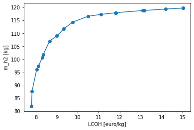
A trade-off exists between minimizing the LCOH and maximizing the hydrogen production.

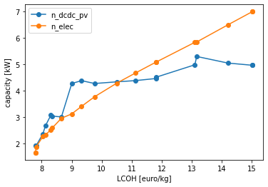
The capacities of the system components increases gradually to improve the hydrogen production, at the expense of an increase in LCOH.

4.2. Robust design optimization

The robust design optimization procedure simultaneously minimizes the mean and standard deviation of a quantity of interest. These statistical moments are quantified following the propagation of the input parameter uncertainties. The stochastic input parameters are characterized in the CASES\H2_FUEL\stochastic_space.csv file. More information on the construction of stochastic_space.csv is found in The stochastic_space.csv file.

4.2.1. Determination of the polynomial order

Based on the PCE truncation scheme (see Polynomial Chaos Expansion), the number of model evaluations required to construct a PCE for each design sample corresponds to 26, 182 and 910 for a maximum polynomial degree of 1,2 and 3, respectively. The polynomial degree that leads to an accurate expansion is not known a priori and should, therefore, be determined iteratively. We refer to Screening of the design space for more details on this method.

import rheia.UQ.uncertainty_quantification as rheia_uq
import multiprocessing as mp

case = 'H2_FUEL'

n_des_var = 20

var_dict = rheia_uq.get_design_variables(case)

X = rheia_uq.set_design_samples(var_dict, n_des_var)

for iteration, x in enumerate(X):
    rheia_uq.write_design_space(case, iteration, var_dict, x, ds = 'design_space_tutorial.csv')
    dict_uq = {'case':                  case,
               'n jobs':                int(mp.cpu_count()/2),
               'pol order':             1,
               'objective names':       ['LCOH','mh2'],
               'objective of interest': 'LCOH',
               'results dir':           'sample_tutorial_%i' %iteration
               }
    if __name__ == '__main__':
        rheia_uq.run_uq(dict_uq, design_space = 'design_space_tutorial_%i.csv' %iteration)

The functions get_design_variables() and set_design_samples() are used to collect the bounds of the design variables and to generate the samples through Latin Hypercube Sampling, respectively. Then, design_space.csv files are created through write_design_space() – one for each design sample – and a PCE is constructed for each sample. At first, a polynomial degree of 1 is selected for evaluation.

For this tutorial, results were generated in advance and stored in RESULTS\PV_ELEC\UQ\sample_tutorial_0 … \sample_tutorial_19. To determine the worst-case LOO error for the 20 design samples, a post_process_uq class object is instantiated, followed by the call of the get_loo() method:

import rheia.POST_PROCESS.post_process as rheia_pp

case = 'H2_FUEL'

pol_order = 1

my_post_process_uq = rheia_pp.PostProcessUQ(case, pol_order)

result_dirs = ['sample_tutorial_%i' %i for i in range(20)]

objective = 'LCOH'

loo = [0]*20
for index, result_dir in enumerate(result_dirs):
    loo[index] = my_post_process_uq.get_loo(result_dir, objective)

print(max(loo))

For the samples provided within the framework (i.e. \sample_tutorial_0 … \sample_tutorial_19) and a maximum polynomial order 1, the worst-case LOO error is 0.0701. Increasing the polynomial order to 2 and generating the PCE for the same design samples decreases the worst-case LOO error down to 0.0140. For this tutorial, this worst-case LOO error is considered acceptable. Hence, a maximum polynomial degree of 2 is selected for the PCE truncation scheme during the robust design optimization.

4.2.2. Reducing the stochastic dimension

From the 20 samples generated to determine the polynomial order, also the Sobol’ indices can be analyzed. Based on these Sobol’ indices, the stochastic parameters with little contribution to the standard deviation of the \(\mathrm{LCOH}\) can be identified. These parameters can be considered deterministic with a negligible loss in accuracy on the \(\mathrm{LCOH}\) mean and standard deviation during the robust design optimization. The details on this method are provided in Screening of the design space.

For a polynomial order of 2, the stochastic parameters with a negligible Sobol’ index can be identified as follows:

import rheia.POST_PROCESS.post_process as rheia_pp

case = 'H2_FUEL'

pol_order = 2

my_post_process_uq = rheia_pp.PostProcessUQ(case, pol_order)

result_dirs = ['sample_tutorial_%i' %i for i in range(20)]

objective = 'LCOH'

my_post_process_uq.get_max_sobol(result_dirs, objective, threshold=1./12.)

A threshold for the Sobol’ index is set at 1/12 (= 1/number of uncertain parameters). 5 out of 12 stochastic parameters have a maximum Sobol’ index below the threshold, which indicates that these parameters can be considered deterministic without losing significant accuracy on the calculated statistical moments of the LCOH. This reduction results in a decrease of 60% in computational cost, as only 72 model evaluations are required to construct a PCE for 7 uncertain parameters in the current truncation scheme, as opposed to 182 model evaluations with 12 uncertain parameters. Thus, by following this strategy, the 5 parameters with negligible contribution can be removed from stochastic_space.csv.

Warning

As the accuracy of this method depends mainly on the number of design samples considered, the results are only indicative. Therefore, the stochastic parameters with negligible Sobol’ index are not removed automatically. It is suggested to evaluate the feasibility of this result, based on the knowledge of the user on the considered system model. To illustrate, the uncertainty on the annual average ambient temperature has a negligible Sobol’ index. This can be considered realistic, as the ambient temperature only slightly affects the power output of the photovoltaic array.

4.2.3. Run a robust design optimization

After the determination of the polynomial degree and the reduction of the stochastic dimension, the robust design optimization can be performed. The code is similar than for the deterministic design optimization procedure. The details on running a robust design optimization are presented in Run a robust design optimization.

import rheia.OPT.optimization as rheia_opt
import multiprocessing as mp

dict_opt = {'case':                  'H2_FUEL',
            'objectives':            {'ROB': (-1, -1)},
            'stop':                  ('BUDGET', 72000),
            'n jobs':                int(mp.cpu_count() / 2),
            'population size':       20,
            'results dir':           'run_1',
            'pol order':             2,
            'objective names':       ['LCOH', 'mh2'],
            'objective of interest': ['LCOH'],
            }

if __name__ == '__main__':
    rheia_opt.run_opt(dict_opt)

Again, a population of 20 samples is selected. With 72 model evaluations required per design sample, a computational budget of 72000 is selected to reach at least 50 generations. The results for the tutorial are provided in RESULTS\PV_ELEC\ROB\run_tutorial. Similar to the deterministic design optimization, the optimization results can be plotted as follows (note that eval_type has changed into 'ROB'):

import rheia.POST_PROCESS.post_process as rheia_pp
import matplotlib.pyplot as plt

case = 'H2_FUEL'

eval_type = 'ROB'

my_opt_plot = rheia_pp.PostProcessOpt(case, eval_type)

result_dir = 'run_tutorial'

y, x = my_opt_plot.get_fitness_population(result_dir)

plt.plot(y[0], y[1], '-o')
plt.xlabel('LCOH mean [euro/kg]')
plt.ylabel('LCOH standard deviation [euro/kg]')
plt.show()

for x_in in x:
    plt.plot(y[0], x_in, '-o')
plt.legend(['n_dcdc_pv', 'n_elec'])
plt.xlabel('LCOH mean [euro/kg]')
plt.ylabel('LCOH standard deviation [euro/kg]')
plt.show()

The results show a single design, which indicates that there is no trade-off between minimizing the LCOH mean and minimizing the LCOH standard deviation. The optimized design corresponds to a PV DC-DC converter of \(1.68~\mathrm{kW}\) and an electrolyzer array of \(1.68~\mathrm{kW}\). The design achieves an LCOH mean of \(7.78~\mathrm{euro} / \mathrm{kg}_{\mathrm{H}_2}\) and a LCOH standard deviation of \(0.85~\mathrm{euro} / \mathrm{kg}_{\mathrm{H}_2}\).

4.3. Uncertainty quantification

Following the robust design optimization, a single optimized design is characterized that optimizes both mean and standard deviation of the LCOH. The Sobol’ indices for this design can illustrate the main drivers of the uncertainty on the LCOH, which can provide guidelines to effectively reduce the uncertainty by gathering more information on the dominant parameters. To evaluate the Sobol’ indices of this design, the design design variables should be transformed in the following model parameters in design_space.csv:

n_dcdc_pv   par 1.68
n_elec      par 1.68

This file can be saved as e.g. design_space_uq.csv, to avoid losing the configuration for optimization. The uncertainty quantification dictionary is then characterized and evaluated as follows:

import rheia.UQ.uncertainty_quantification as rheia_uq
import multiprocessing as mp

dict_uq = {'case':                  'H2_FUEL',
           'n jobs':                int(mp.cpu_count()/2),
           'pol order':             2,
           'objective names':       ['lcoh','mh2'],
           'objective of interest': 'lcoh',
           'draw pdf cdf':          [True, 1e5],
           'results dir':           'opt_design_tutorial'
           }

if __name__ == '__main__':
    rheia_uq.run_uq(dict_uq, design_space = 'design_space_tutorial_uq.csv')

For this tutorial, the results of the uncertainty quantification are provided in RESULTS\PV_ELEC\UQ\opt_design_tutorial

The resulting Sobol’ indices can be plotted in a bar chart:

import rheia.POST_PROCESS.post_process as rheia_pp
import matplotlib.pyplot as plt

case = 'H2_FUEL'

pol_order = 2

my_post_process_uq = rheia_pp.PostProcessUQ(case, pol_order)

result_dir = 'opt_design_tutorial'

objective = 'lcoh'

names, sobol = my_post_process_uq.get_sobol(result_dir, objective)

plt.barh(names, sobol)
plt.show()

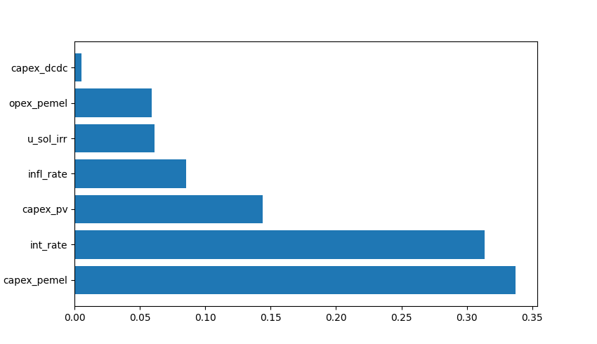
The Sobol’ indices illustrate that the uncertainty on the interest rate and the investment cost of the PV array and electrolyzer stack dominate the uncertainty on the LCOH.

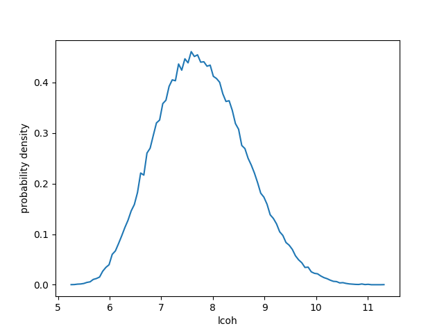
Finally, the probability density function is plotted with the get_pdf() method:

x_pdf, y_pdf = my_post_process_uq.get_pdf(result_dir, objective)

plt.plot(x_pdf, y_pdf)
plt.xlabel('lcoh')
plt.ylabel('probability density')
plt.show()