5.1. Robust optimization of a power-to-power system

The robust design optimization of the Levelized Cost Of Electricity for a hydrogen-based power-to-power system for a dwelling in Belgium.

In this first example, a robust design optimization is performed on a grid-connected household in Brussels, supported by a photovoltaic-hydrogen system. To optimize the system, 4 design variables are considered: the photovoltaic array capacity, electrolyzer stack capacity, fuel cell stack capacity and hydrogen tank capacity. The mean and standard deviation of the Levelized Cost Of Electricity (LCOE) are selected as objectives. The CAPEX, OPEX, replacement cost and lifetime of the components are considered uncertain, as well as the wholesale electricity price, electricity demand, interest rate and inflation rate. A detailed illustration of the energy system model and the stochastic space is provided in Power-to-power.

After 150 generations, a trade-off exists between minimizing the LCOE mean and LCOE standard deviation:

import rheia.POST_PROCESS.post_process as rheia_pp
import matplotlib.pyplot as plt

case = 'H2_POWER'

eval_type = 'ROB'

my_opt_plot = rheia_pp.PostProcessOpt(case, eval_type)

result_dir = 'run_tutorial'

y, x = my_opt_plot.get_fitness_population(result_dir)

plt.plot(y[0], y[1], '-o')
plt.xlabel('LCOE mean [euro/MWh]')
plt.ylabel('LCOE standard deviation [euro/MWh]')
plt.xticks([y[0][0], y[0][-1]])
plt.yticks([y[1][0], y[1][-1]])
plt.show()

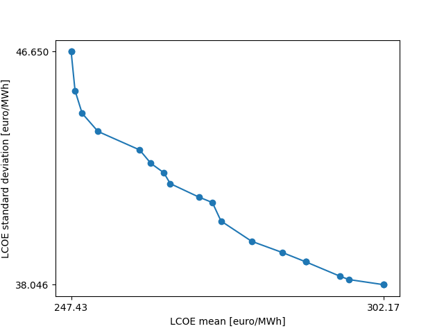
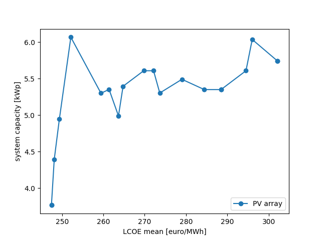
The Pareto front illustrates a trade-off between minimizing the LCOE mean and LCOE standard deviation. This means that no single design exists that simulateounsly achieves the minimum LCOE mean and minimum LCOE standard deviation. The optimized LCOE mean design achieves an LCOE mean of 247 euro/MWh and a LCOE standard deviation of 46 euro/MWh. Instead, the robust design (i.e. the design with the lowest standard deviation) achieves an LCOE mean of 302 euro/MWh and a LCOE standard deviation of 38 euro/MWh. The designs that correspond to this Pareto front have the following PV array capacity:

plt.plot(y[0],x[0],'-o')
plt.xlabel('LCOE mean [euro/MWh]')
plt.ylabel('system capacity [kWp]')
plt.legend(['PV array'])
plt.show()

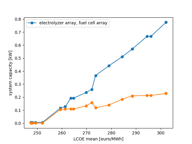
Electrolyzer array and fuel cell array capacity:

for x_in in x[1:3]:
    plt.plot(y[0],x_in,'-o')

plt.xlabel('LCOE mean [euro/MWh]')
plt.ylabel('system capacity [kW]')
plt.legend(['electrolyzer array, fuel cell array'])
plt.show()

Hydrogen storage tank capacity:

plt.plot(y[0],x[3],'-o')
plt.xlabel('LCOE mean [euro/MWh]')
plt.ylabel('system capacity [kWh]')
plt.legend(['storage tank'])
plt.show()

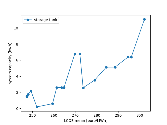
These results indicate that the optimized LCOE mean is achieved by a PV array. In order to improve the robustness of the LCOE, the optimizer gradually increases the electrolyzer, fuel cell and storage tank capacity.